Analysis of fires detected in the Paraná River delta, Argentina, using VIIRS product data. Part 2.

In the second part of this guide, we will delve deeper into the dataset obtained in the first part and conduct additional processing and visualization. This will enable us to analyze the temporal and spatial patterns of fire occurrences in our study area from 2012 to 2021. By doing so, we aim to gain valuable insights into the fire phenomena in the Parana River Delta while raising further questions that will be addressed in future guides using various techniques and additional data.

As we discussed in the first part of this guide, the data chosen to perform this analysis was VIIRS Active Fire product data because of its association with fires. For more information about the study area and the criterias that we’re taking into consideration in this guide, please refer to part 1.

Methodology

The processing of the dataset obtained in the first part of this guide will be performed using Python and basic data analysis libraries such as Numpy, Pandas, Matplotlib, among others. More specific libraries will be used, such as Geopandas, which is highly useful for the analysis of georeferenced data. In addition to these pre-processed VIIRS data, vector layers files will be also utilized for the study area delimitation.

All the data and vector layers files were obtained from public access repositories. Finally, the implementation of the analysis was designed to be carried out in the Google Colaboratory environment with the aim of making it easier to perform for anyone interested

Step-by-step Guide for Data Processing and Analysis in Python

Libraries and functions

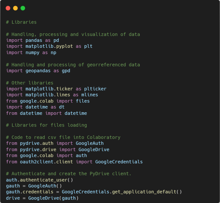
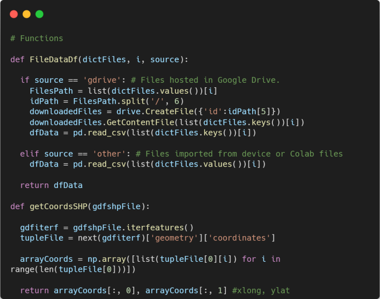
Firstly we need to import libraries, such as standard libraries for the analysis of data  and necessary libraries to access files stored in Google Drive, in case you prefer working in this way. Additionally we need to load functions that will be used later on.

Data Loading

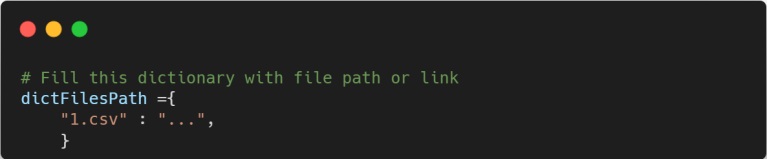
Unlike what was done in the first part of this guide, now we will load the dataset previously obtained. Again, to load the file with the data we are going to work with, we will create a dictionary in which the key will be a generic name for the csv file, while the key value will be the link/path of the file as the case may be. Keep in mind that this file can be uploaded from Google Drive or from your own device directly on Colab.

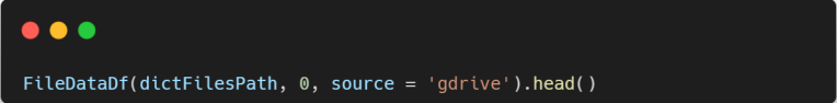
Before creating our dataframe with data for further analysis, let’s check if the data loads as we expect and datatypes are correct. For more information on the columns that should be expected to be loaded, refer to the first part of this guide.

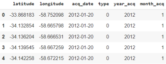
Once confirmed data loads correctly, we can proceed to create the pandas dataframe using the code provided below.

Prior to continuing with the analysis of data, let’s get basic info from our dataset recently loaded.

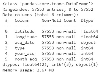
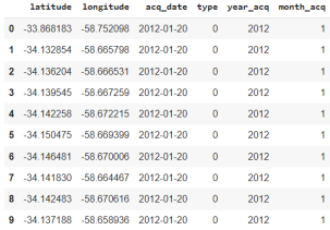
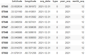
As we can observe, the loaded dataframe consists of 57552 entries corresponding to the filtered data from our original VIIRS product dataset of detected hotspots. The first entry is from March 2012, while the last one is from December of 2021. This dataset is the result of initial processing and modifications made to the original one. These modifications included the removal of certain columns and the addition of others that are particularly useful for this part, such as “year_acq” and “month_acq”. After verifying that everything has been loaded correctly, we can proceed with the next steps.

Data visualization and analysis of fire occurrence phenomena

The focus of the following analysis is to study the temporal occurrence and spatial distribution of the detected hotspots in the study area between 2012 and 2022. However, you can come up with your own ideas to focus your analysis and obtain your own insights from either the original or the processed dataset.  

Processing of data before visualization

If you haven’t noticed before, there are multiple entries for each day, corresponding to different hotspots detected within our study area. You can verify this by examining the columns corresponding to the coordinates associated with each entry, “latitude” and “longitude”. Therefore, the first step to perform is to count the number of hotspots per day, independently of their geographic position.

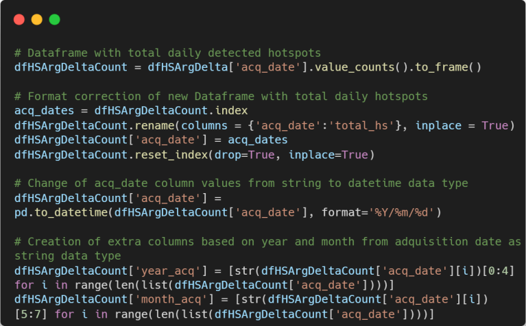
It’s worth noting from above that we had to include some additional code to reformat the data and recreate certain columns that were deleted during previous processing stages. These columns will be essential for our subsequent analysis.

Let’s examine the output of the newly created dataframe that contains the total number of hotspots detected per day. Commands .info() and .head() show us how different this new dataframe is compared with the previous one.

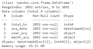
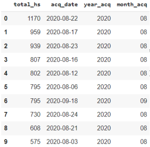
The result of the processing is a new dataframe. Now, instead of having an entry for every hotspot detected by day, we have the total hotspots detected by day as a row value in the column “total_hs”. The original dataframe has been significantly reduced from 57552 to 2092 rows. Additionally, the data type of “acq_date” column values were converted to datetime.

Analysis of temporal fire occurrence

As a first approach for analyzing the occurrence of fires in our study area during the selected period of time is to create a time series plot of the total number of hotspots detected each day. This will provide us with an initial understanding of the frequency and pattern of fires.

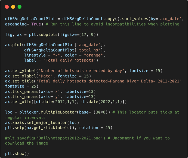
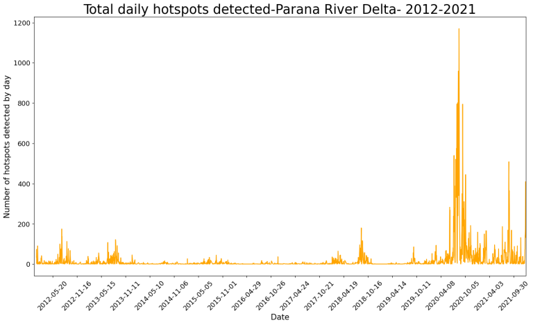
This plot displays the total detected hotspots for each day between May 20th, 2012 and December 31th, 2021. It allows us to analyze various aspects of the occurrence of fires in our study area during the selected time period. One of this aspects is that there were extended periods with few or no fires, as well as periods with a higher frequency. Additionally, not all periods had the same number of detected hotspots, with some having a higher frequency of fires than others. Between these periods there where two notable periods with a high frequency of fires are the peaks in 2020 and 2021. Other interesting peaks occurred in 2012, 2013 and 2018. 

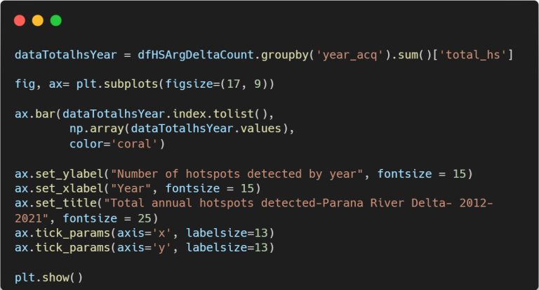
To continue with the analysis, let’s take a closer look at the three years with the highest frequency of fires (years with the highest peaks). Because of the irregular distribution of fires throughout the year, as shown in the plot, it’s challenging to identify if 2012, 2013 or 2018 had the highest number of fires. To address this, we can further our analysis with a bar plot that shows the total number of hotspots detected by year.

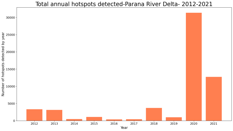
The latest bar plot provides us further insight into the interpretation of the first plot. Since each bar shows the total detected hotspots for a given year, regardless of at which month it occurred, it’s easier to identify which years had the highest frequency of fires. However, this plot doesn’t definitively identify the year with the third highest frequency of fires, apart from 2020 and 2021. To clarify this, we can delve deeper into the dataframe used to create the bar plot.

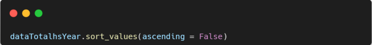
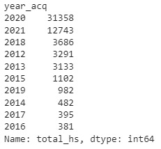
Finally, after analyzing the dataframe shown above, we can confirm that the three top years with the highest number of detected hotspots were 2018, 2020 and 2021. With this information we can continue with a more detailed examination. First, we will explore the occurrences of fires throughout the year for each of these years. Then, we will identify the top five days with the highest number of detected hotspots for these three years. Note that the number of top years and days were chosen arbitrarily. You can choose your own top including more years and days, depending on your criteria.

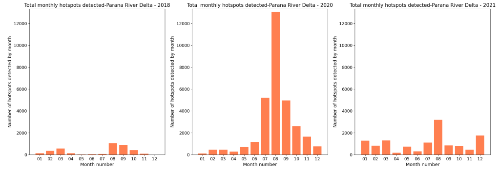
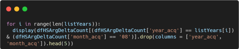
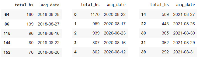
Upon examining the output from the previous code, we can draw some interesting conclusions. Firstly, it’s worth noting that the month with the highest number of fires detected in all three years was the month number 08, August. This reinforces what we already knew about our study area, that fires tend to occur towards the end of winter. Secondly, it’s also interesting to observe that the total number of fires in 2020 was much higher than in the other years with, for example, a 1:10 ratio for August 2018. Thirdly, unlike what happened in 2018 and 2020, the fire activity in 2021 in the study area was relatively constant throughout the year. Lastly, after reviewing the tables for the top five days with the highest number of detected hotspots, it becomes evident that most of the days fell in the period within the last 10 days of August.

Analysis of spatial distribution of fires

Now, we can leverage the full potential of our georeferenced dataset to create more interesting plots. Building upon our previous analysis, where we identified the years, months, and specific days with the highest number of detected hotspots, let’s explore the spatial distribution of these hotspots in our study area. 

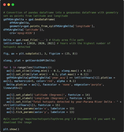
To begin, we will plot all the hotspots detected during the top three years with the highest occurrences of fires separetely. This will provide us with a visual representation of the geographic spread of these fires.

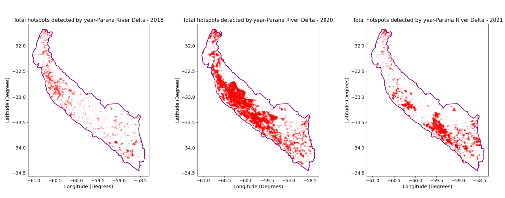
These plots provide us insights into the spatial distribution of the fires detected during the chosen years. Despite being the top three years, the number of detected hotspots varies among them, which is evident in the plots shown before. In 2018, the fires were dispersed throughout the study area, with a higher concentration in the upper region. In 2020, the fires occurred in almost every part of the River Parana Delta, but the density was relatively lower in the bottom section. In 2021, we can observe a higher density on the middle and lower regions, with a concentrated area of maximum intensity. 

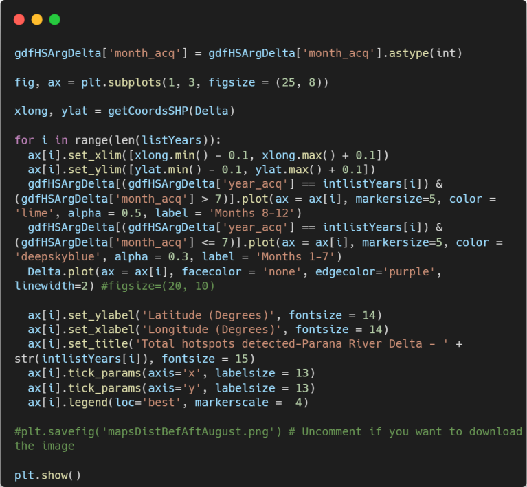
While the previous plots show us the overall spatial distribution of fires throughout the year, it is important to note that the fire occurrence in the study area is not uniform. As we discovered earlier, the peak of hotspot detection for all three years falls in August, the month number eight. Now, let’s explore deeper into the spatial distribution by analyzing the number of fires detected before and after August, including August itself.

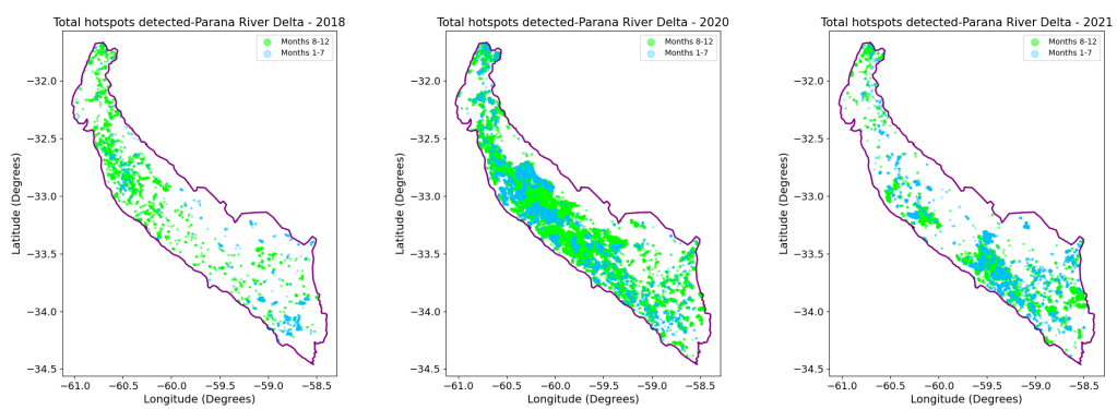
As we discussed before, the fires occur towards the end of the winter to facilitate grass regrowth for pasture. The preceding plots confirm this and provide some extra valuable insights for our analysis. According to the plots, in 2018 and 2020 the highest number of fires occurred during months 8 to 12. However, there were differences in their distribution pattern. On the other hand, for 2021 we can observe that fires in months 1-7 were significantly important, almost equaling the ones that occurred in months 7-12. This supports what we observed in the bar plot made before for this year.

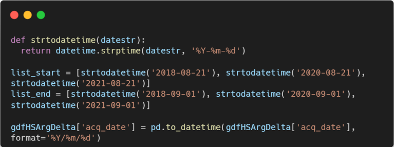
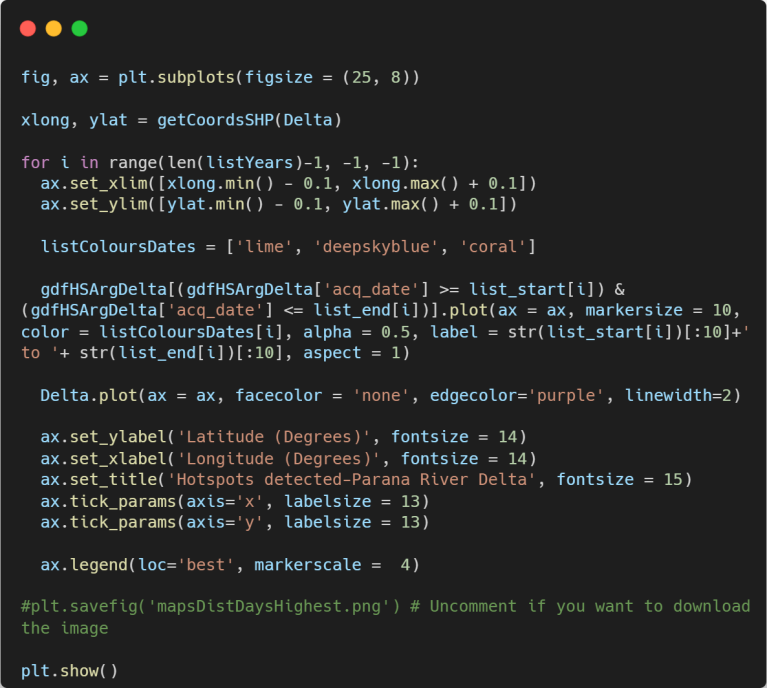
To conclude our analysis, we can incorporate an additional visualization. We will examine the distribution of hotspots detected during the last ten days of August in 2018, 2020 and 2021. The idea is to attempt to identify any patterns during the days found as the ones with the highest number of fires detected in our study period.

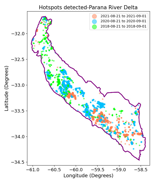
From the last plot we can observe that when comparing the same period of days for the three years, there is no consistent pattern in spatial distribution of the fires. For example, one might expect to find a similarity in the locations where the fires occurred, with a superposition of all the detected hotspots. This was not the case for the years and the period chosen. However, what becomes evident is that each year exhibits distinct clusters of fires of different sizes, which may have originated from independent initial fire sources and subsequently expanded.

After this final analysis, one question arises: what factors contributed to this particular behavior during the days identified as the ones with the highest number of fires? While most of the fires in our study area have a human cause, it would be interesting to understand why these fires originated in specific locations rather than in other areas.

Conclusions

Throughout this post, divided in two parts, we have worked with a VIIRS Active Fire product dataset obtained from the NASA-FIRMS website for our study area and a specific time period. In the first part we did a preliminary processing and extracted the relevant data of interest. In the second part we conducted an additional processing to visualize the dataset obtained in the first part. This enabled us to gain valuable insights into the occurrence of fires in the Parana River delta and address different questions about this, while also uncovering new ones. 

One of the questions addressed in this post pertains to the identification of the three years, from 2012 to 2021, with the highest number of detected fires. Additionally, we explored the temporal distribution of the fires throughout the year for these specific years. Then, through further processing and analysis, we were able to identify the exact day with the highest number of fires during the aforementioned time period. 

Another significant aspect of this analysis involved the spatial distribution of fires. We examined how the detected fires were spatially distributed during the three years with the highest number of occurrences. This allowed us to observe similarities and differences among these years.

Finally, one question arose: What factors caused the initial location of the fire clusters found in August for 2018, 2020 and 2021? Was it solely due to anthropogenic causes? Were the weather conditions or the hydrology?  Or was it a combination of all of these factors? These questions will be explored in future posts.

Sources

Salvia, M. M. (2010). Aporte de la teledetección al estudio del funcionamiento del macrosistema Delta del Paraná: análisis de series de tiempo y eventos extremos.

Instituto Nacional del Agua, INA. (2018). Delta del Paraná: Proyectos Estratégicos para el Desarrollo Sustentable. Informe 01: “Base de datos Georeferenciada del Delta de Paraná”.

Links to repositories

VIIRS Active Fire product data: https://firms.modaps.eosdis.nasa.gov/download/

Paraná River delta borders vector file: https://www.google.com/maps/d/u/0/viewer?mid=1_ArYZsWx-IvFCsNuXA-Z0u60vVcVLP76&ll=-35.24217356383713%2C-59.32243393359376&z=6
*Note: In this site you can get the layer as a KML file. After download, convert into a .shp file.

Argentina borders vector file: https://www.ign.gob.ar/NuestrasActividades/InformacionGeoespacial/CapasSIG
*Note: Select the layer named “pais” with geometry “poligono” (polygon).

Github repository of this project: https://github.com/francobarrionuevoenv21/codeforenviroprojects/tree/VIIRS_fires_Delta